Introduction: Why Think About Energy?
Imagine that you want to teach a machine to distinguish between a "cat" and a "dog." The usual approach is to tell it: "Look at this image and tell me what it is." After seeing thousands of images, the machine learns to say "cat" or "dog." But a fundamental question remains: Does the machine really understand how compatible this image is with a cat?
This is where Energy-Based Models, or EBMs, come in. The idea is simple but deep: instead of directly saying "this is a cat," we assign a number to each combination of input and output that measures their compatibility. We call this number Energy.
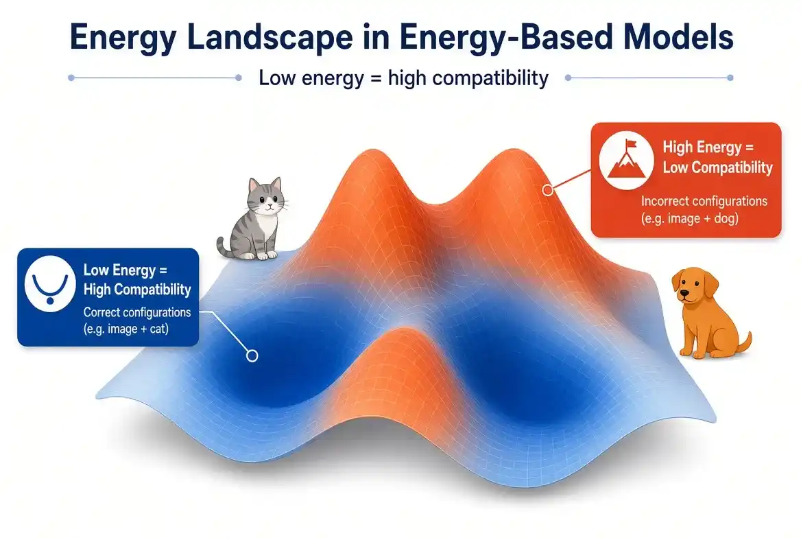
Low energy = high compatibility
High energy = low compatibility
So instead of merely producing a label, the machine can say: "The combination of this image with the label cat has energy 0.2, while the combination with dog has energy 8.5; therefore, cat is more compatible."
This shift in perspective opens a world in which decision-making, learning, latent variables, and efficient inference can all be studied within an energy-based framework.
Part One: The Energy Function — The Heart of an EBM
1.1 A Simple but Powerful Definition
Suppose we have two sets of variables: X (the input, what we observe) and Y (the output, what we want to predict). We define an energy function as:
This function assigns a real number to each pair (x,y). The smaller the number, the more compatible the configuration is considered.
1.2 Inference: Finding the Best Y
Once we have the energy function, inference means finding the Y with the lowest energy:
In other words: "Among all possible Y values, find the one that has the lowest energy for the observed X."
1.3 Learning: Shaping the Energy Landscape
Learning in an EBM means finding an energy function that:
- Assigns lower energy to correct configurations.
- Assigns higher energy to incorrect configurations.
This process can be viewed as shaping the Energy Landscape. Imagine a mountain range with deep valleys and high peaks. Desirable configurations occupy low-energy regions, while undesirable configurations occupy high-energy regions.
Part Two: The Four Pillars of EBM
In A Tutorial on Energy-Based Learning, LeCun and colleagues describe four main components involved in building and training an EBM:
| Component | Explanation |
|---|---|
| Architecture | The internal structure of the energy function E(W, Y, X) |
| Inference Algorithm | A method for finding Y with minimum energy |
| Loss Function | A criterion for shaping the energy function appropriately |
| Learning Algorithm | A method for finding the parameters W |
2.1 Loss Function: Which Loss Is Good?
Not all loss functions behave in the same way. Some may lead to collapse, where the energy function fails to maintain a meaningful distinction between correct and incorrect configurations. Here are the main loss families discussed in this framework.
a) Energy Loss — Simple but Dangerous
This only lowers the energy of the correct answer. The problem is that it does not explicitly force incorrect answers to have higher energy. In some high-capacity settings, this can lead to collapse.
b) Perceptron Loss — Without a Margin
This loss compares the energy of the correct answer with the lowest-energy answer found by the model. But it does not impose an explicit margin, so correct and incorrect configurations may remain only slightly separated.
c) Margin Losses — With a Safety Gap
The idea is that the correct answer should have energy at least m lower than a relevant incorrect answer:
Here Ȳi is a relevant incorrect answer, often the Most Offending Incorrect Answer with the lowest energy.
Hinge Loss, Log Loss, LVQ2, MCE, Square-Square, and Square-Exponential are discussed within this family of margin-based criteria.
d) Negative Log-Likelihood (NLL) — A Probabilistic View
This loss follows from the Gibbs-Boltzmann interpretation and, when the corresponding probability distribution is properly defined, relates to maximizing conditional probability P(Y|X). The main difficulty is the Partition Function: the integral or sum over the entire output space, which can be extremely large or intractable.
Part Three: Latent Variables — When Something Is Not Observed
3.1 Why Do We Need a Latent Variable?
Suppose we want to build a face detection system. We want to know whether a face exists in the image (Y), but we do not know the face location (Z). This Z is a Latent Variable.
The energy function now becomes:
Inference can then be written jointly over Y and Z:
For a deeper treatment of this topic, see Latent Variables and Yann LeCun's Path Toward Autonomous AI .
3.2 Free Energy — Marginalization Instead of Simple Minimization
Sometimes, instead of selecting only the best Z, we want to consider multiple values of Z. This is where Free Energy enters:
In the zero-temperature limit, that is, as β → ∞, this expression approaches the minimum energy over z, under suitable conditions.
3.3 Multiple Possible Answers for One Input
One important property of a latent variable is that changing Z can allow the model to represent multiple possible outputs for the same X:
├── Z₁ → Y₁
├── Z₂ → Y₂
├── Z₃ → Y₃
└── Z₄ → Y₄
For example, a video scene can have several possible futures. A sentence can have multiple valid translations. A latent variable can therefore provide a way to represent this multimodality.
Part Four: Efficient Inference — Factor Graphs
4.1 The Large Search Space Problem
If Y is an image, its state space is enormous. If Y is a sentence, the number of possible sequences is also huge. How can we find the minimum-energy configuration efficiently?
4.2 The Solution: Factorization
The idea of a Factor Graph is to decompose the energy into several factors, each depending only on a subset of the variables:
Ea(X, Z₁)
+ Eb(X, Z₁, Z₂)
+ Ec(Z₂, Y₁)
+ Ed(Y₁, Y₂)
This structure can allow us to use Dynamic Programming and search for optimal paths in a trellis more efficiently than enumerating all possible configurations.
4.3 Key Algorithms
- Min-Sum Algorithm: Used to find minimum-cost configurations in structured models; in chains, it is closely related to the idea behind Viterbi.
- Forward Algorithm: Used to sum path weights and compute quantities such as partition functions in appropriate models.
- A*: A guided search method useful in some large state spaces.
These algorithms are part of what makes EBMs practical for structured problems such as speech, handwriting, and sequence modeling.
Part Five: EBM vs Probabilistic Models
5.1 Turning Energy into Probability
When the necessary normalization conditions hold, we can construct a probability distribution from energy:
But this creates two main challenges:
- The energy function must satisfy the conditions needed for convergence and normalization.
- Computing the partition function can be extremely expensive in large spaces.
5.2 The EBM Advantage: Normalization Is Not Always Needed for Decision-Making
LeCun emphasizes that if the final goal is decision-making, we do not necessarily need a normalized probability. If all we want is the best decision, comparing Energy values may be sufficient.
In LeCun's framework, probabilistic models can be interpreted within the broader Energy-Based Model framework; not every EBM is necessarily a normalized probabilistic model.
5.3 The Label Bias Problem
In some graph-based models with local normalization, including certain sequence models, local normalization can lead to Label Bias; that is, output structures with different numbers of possible paths can be affected by how probabilities are normalized locally.
An energy-based approach with Late Normalization can reduce this limitation by assigning a score or Energy to the whole structure first and, when needed, performing normalization at the global level.
Part Six: EBM for Sequences and Structured Outputs
6.1 Linear Structured Models
In problems such as Sequence Labeling, Y is a sequence of labels. In a model that is linear in its parameters, the energy can be written as:
where F(X,Y) is a feature vector. Models such as CRFs, SVMMs, and MMMs can be interpreted within the broader Energy-Based Learning framework.
6.2 Nonlinear Graph-Based Models
Factors can also be built using neural networks. This allows the model to learn more complex nonlinear relationships and use deep learning components to model different parts of a structured graph.
6.3 Graph Transformer Networks
GTN, in the framework discussed by LeCun and colleagues, is a hierarchical architecture in which:
- Graphs are used as data structures.
- Each module takes a graph and can produce another graph.
- Parameters are trained using back-propagation and gradient-based optimization with graph and trellis structures.
For example, in handwritten word recognition, an image can first be transformed into a segmentation graph and then into higher-level interpretive graphs, with algorithms such as Viterbi used to find the best path.
Part Seven: A Practical View — From EBM to JEM
7.1 Why Can EBMs Be Difficult in Practice?
EBMs are highly flexible in theory, but in practice:
- Training can be sensitive.
- MCMC can be expensive.
- Hyperparameters matter significantly.
- Sampling or optimization can become unstable.
7.2 Sampling with Langevin Dynamics
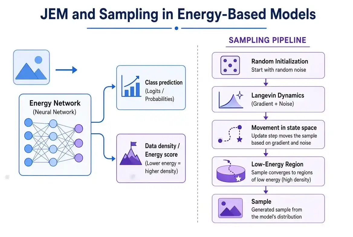
To generate samples from a generative EBM, we can use MCMC methods such as Langevin Dynamics:
↓
Energy Model
↓
Gradient + Noise
↓
Movement in State Space
↓
Low-Energy Region
↓
Sample
Langevin Dynamics is not simply gradient descent; it also includes a random component, which is why it belongs to the MCMC family.
7.3 Sampling Buffer
To reduce sampling costs, practical implementations such as JEM can maintain previous samples in a Replay Buffer and use them as starting points for later chains.
In some JEM settings, a 5% random reinitialization probability is used. This is a specific implementation strategy, not a general definition of EBMs.
7.4 JEM — Joint Energy Model
JEM (Joint Energy Model), introduced by Grathwohl and colleagues, shows how a classifier can be reinterpreted as an energy-based model for the joint distribution P(X,Y), while still representing the conditional classification problem.
├── Class
└── Data Density
In JEM, the same network can support both discriminative modeling and generative energy-based modeling.
Its training therefore has two aspects:
- Classification Loss using Cross Entropy
- Generative Maximum Likelihood with approximate gradients based on SGLD / MCMC
Therefore, it is more precise not to call the second part directly a "Contrastive Divergence Loss"; in JEM, the generative likelihood gradient is approximated through MCMC/SGLD.
For a broader connection between EBM, JEPA, latent variables, and LeCun's later ideas, see EBM and JEPA in Yann LeCun's Perspective .
Part Eight: Anomaly Detection and Generation
8.1 Anomaly Detection
In an EBM that has genuinely been trained to model the data distribution:
→ Greater compatibility with the modeled distribution
High Energy
→ Greater incompatibility with the modeled distribution
Therefore, Energy can be used as a score for identifying unusual or Out-of-Distribution samples; however, this relationship is not a universal law for every EBM.
8.2 Generation
↓
Langevin / MCMC
↓
Energy ↓
↓
Sample
In this setting, the Energy Model can indirectly act as a generator. The model does not directly draw the image itself; instead, it defines a landscape that guides the sampler toward low-energy regions.
Part Nine: EBM in One View
X → Y ?
↓
Instead of directly producing Y,
define an Energy for each X,Y configuration.
↓
E(Y, X)
↓
Lowest Energy = Best Answer
↓
Now we need to learn the Energy function.
↓
Loss Function
↓
Correct → Lower Energy
Wrong → Higher Energy
↓
What if some variables are not observed?
↓
Latent Variable Z
↓
What if outputs are structured and numerous?
↓
Factor Graph
↓
What if they are sequences?
↓
Structured EBM
↓
What if they become more complex?
↓
Neural Networks + Graphs + GTN
↓
And what if exact inference is difficult?
↓
Approximate Inference / Sampling
Final Thoughts: Why Are EBMs Important?
EBM is a broader framework than probabilistic models. Within it:
- We do not necessarily need to turn the model into a normalized probability distribution for decision-making.
- We can use an Energy function to express the compatibility of configurations.
- We can introduce latent variables into the model.
- We can represent multiple possible states for one input.
- We can use inference and sampling to search through a state space.
- In models such as JEM, one network can support both discriminative and energy-based roles.
"All models are wrong, but some are useful." — George Box
EBMs encourage us to think about compatibility instead of insisting on directly producing one answer; to model Energy instead of always starting with a normalized probability; and to consider a space of possible answers instead of assuming a unique outcome.
From here, the path leads to larger ideas such as Latent Variables, Multiple Prediction, World Models, and JEPA. EBM is not one specific model, but a common framework and language for expressing compatibility, inference, and decision-making.
For the broader conceptual context of autonomous intelligence and World Models, see Yann LeCun's Autonomous Machine Intelligence Architecture and World Models and Yann LeCun's Philosophy of Intelligence .
Frequently Asked Questions About EBM, Latent Variables, JEM and JEPA
What is an Energy-Based Model (EBM)?
An Energy-Based Model assigns an energy value to configurations of variables. Lower energy represents greater compatibility within the learned model, while higher energy represents lower compatibility.
What is the main idea behind an EBM energy function?
The energy function maps a configuration, such as an input-output pair, to a scalar value. Inference can then search for a configuration with minimum energy rather than directly predicting one answer through a normalized probability distribution.
How does inference work in an Energy-Based Model?
In its simplest form, inference searches for the value of the output that minimizes the energy function. For structured or very large output spaces, the inference process may require specialized algorithms or approximate methods.
What is a latent variable in an EBM?
A latent variable is a variable that is not directly observed or labeled but can explain hidden structure in the problem. In an EBM, latent variables can be included in the energy function and optimized or marginalized during inference.
What is the difference between Energy-Based Models and probabilistic models?
A probabilistic model explicitly defines a normalized probability distribution. An EBM can instead focus on assigning relative compatibility through energy values, and normalization is not necessarily required when the task is direct decision-making.
What is Free Energy in a latent-variable EBM?
Free Energy provides a way to account for multiple possible latent-variable configurations instead of selecting only one latent state. Under suitable conditions and limits, it is related to minimizing or marginalizing over the latent variables.
Does every EBM require MCMC or Langevin Dynamics?
No. MCMC and Langevin Dynamics are especially relevant when sampling or approximate inference is needed. Some EBMs can use optimization-based inference or exact algorithms for particular structured problem classes.
What is JEM?
JEM, or Joint Energy Model, is an approach that interprets a classifier as an energy-based model over the joint relationship between inputs and labels. It can support both discriminative classification and an energy-based view of data density.
What is the relationship between EBM and JEPA?
EBM provides a general framework for expressing compatibility and energy, while JEPA is a joint-embedding predictive architecture built around prediction in representation space. They are related to broader ideas about latent representations, prediction, and autonomous intelligence, but they are not identical concepts.
How are EBM, latent variables and World Models connected?
Latent variables can represent hidden states, while World Models attempt to represent and predict meaningful aspects of an environment. Energy-based formulations can provide one way of describing compatibility among possible states or configurations. For further reading, see Latent Variables and Yann LeCun's Path Toward Autonomous AI and World Models and Yann LeCun's Philosophy of Intelligence .
Can energy be used for anomaly detection?
It can be used as a scoring mechanism in EBMs that are actually trained to model data compatibility or density. However, a low or high energy value should not automatically be interpreted as normal or anomalous for every possible EBM without considering how the model was trained and what its energy represents.
Where should I start if I want to study EBM more deeply?
A useful path is to begin with the energy function and inference, then study latent variables and Free Energy, structured inference, sampling and JEM, and finally move toward related ideas such as World Models, autonomous machine intelligence, and JEPA.
EBM also connects to broader questions about reasoning and gradient-based learning. A related discussion is available in Reasoning and Gradient-Based Learning in Yann LeCun's View .
To place EBM inside the broader AI landscape, see AI Through Multiple Lenses: A Personal Overview .
Key EBM Glossary
| Term | Persian Equivalent | Short Explanation |
|---|---|---|
| Energy Function | تابع انرژی | A function assigning a scalar compatibility value to a configuration |
| Inference | استنتاج | Finding a configuration with minimum Energy |
| Energy Landscape | چشمانداز انرژی | The shape of the Energy function over the state space |
| Loss Function | تابع زیان | A function used to shape the Energy function |
| Collapse | فروپاشی | A situation where Energy fails to preserve meaningful distinctions |
| Margin | حاشیه | The required separation between correct and incorrect answers |
| Latent Variable | متغیر پنهان | A variable whose true value is not directly observed or labeled during training |
| Free Energy | انرژی آزاد | A function that accounts for a collection of latent-variable values |
| Factor Graph | گراف عاملی | A representation that decomposes an energy function into smaller factors |
| Most Offending Incorrect Answer | بدترین پاسخ نادرست | The incorrect answer with the lowest energy among the considered wrong answers |
| NLL | لگاریتم درستنمایی منفی | A probabilistic loss based on likelihood |
| MCMC | زنجیرهی مارکوف مونتکارلو | A family of sampling methods |
| Langevin Dynamics | دینامیک لانژوین | An MCMC method combining gradient information and random noise |
| SGLD | گرادیان تصادفی لانژوین | A stochastic-gradient version of Langevin sampling |
| Replay Buffer | بافر بازپخش | A buffer of previous samples used to initialize later chains |
| JEM | Joint Energy Model | An interpretation of a classifier as a joint energy model |
| GTN | Graph Transformer Network | A hierarchical graph-based architecture in the structured EBM framework |
| CRF | میدان تصادفی شرطی | A structured probabilistic model |
| SVMM | ماشین مارکوف بردار پشتیبان | A margin-based structured model |
| MMMN | Maximum Margin Markov Network | A Markov model trained with margin-based criteria |
| Perceptron Loss | زیان پرسپترون | A comparative loss without an explicit margin |
| Hinge Loss | زیان لولایی | A margin-based loss |
| Square-Square Loss | زیان مربع-مربع | One of the loss functions discussed in the EBM framework |
| Square-Exponential Loss | زیان مربع-نمایی | One of the loss functions discussed in the EBM framework |
References & Further Reading
- LeCun, Y., Chopra, S., Hadsell, R., Ranzato, M. A., & Huang, F. J. (2006). A Tutorial on Energy-Based Learning. In Predicting Structured Data. MIT Press. https://yann.lecun.org/exdb/publis/pdf/lecun-06.pdf
- Dawid, A., & LeCun, Y. (2024). Introduction to Latent Variable Energy-Based Models: A Path Towards Autonomous Machine Intelligence. Journal of Statistical Mechanics: Theory and Experiment, 2024, 104011. DOI: 10.1088/1742-5468/ad292b
- Grathwohl, W., Wang, K.-C., Jacobsen, J.-H., Duvenaud, D., Norouzi, M., & Swersky, K. (2020). Your Classifier is Secretly an Energy Based Model and You Should Treat it Like One. ICLR. https://arxiv.org/abs/1912.03263
- Ha, D., & Schmidhuber, J. (2018). World Models. arXiv preprint.
- Hafner, D., et al. (2019). Learning Latent Dynamics for Planning from Pixels. ICML.
- Assran, M., et al. (2023). Self-Supervised Learning From Images With a Joint-Embedding Predictive Architecture. CVPR.
- Kingma, D. P., & Welling, M. (2014). Auto-Encoding Variational Bayes. ICLR.
This article is my attempt to tell the story of EBM from my own perspective; a story that begins with a simple number for measuring compatibility and leads to inference, latent variables, sampling, structured modeling, and eventually to broader ideas such as World Models and JEPA.